Face-centred cubic (FCC)#
Pearson symbol: cF
Face-centered cubic lattice is described by the class FCC.
It is defined by one parameter: \(a\) with conventional lattice:
\[ \begin{align}\begin{aligned}\boldsymbol{a}_1 = (a, 0, 0)\\\boldsymbol{a}_2 = (0, a, 0)\\\boldsymbol{a}_3 = (0, 0, a)\end{aligned}\end{align} \]
And primitive lattice:
\[ \begin{align}\begin{aligned}\boldsymbol{a}_1 = (0, a/2, a/2)\\\boldsymbol{a}_2 = (a/2, 0, a/2)\\\boldsymbol{a}_3 = (a/2, a/2, 0)\end{aligned}\end{align} \]
Variations#
There are no variations for face-centered cubic lattice.
One example is predefined: fcc with \(a = \pi\).
Example structure#
Default kpath: \(\Gamma-X-W-K-\Gamma-L-U-W-L-K\vert U-X\).
Picture |
Code |
|---|---|
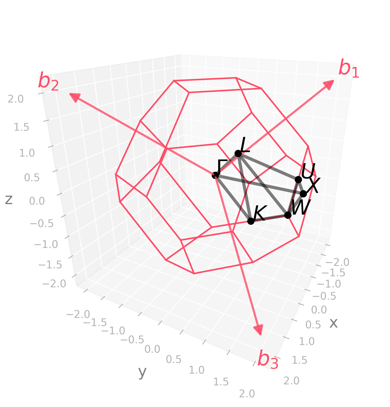
|
import radtools as rad

l = rad.lattice_example(f"FCC")
l.plot("brillouin-kpath")
# Save an image:
l.savefig(
    "fcc_brillouin.png",
    elev=23,
    azim=28,
    dpi=300,
   bbox_inches="tight",
)
# Interactive plot:
l.show(elev=23, azim=28)
|
Picture |
Code |
|---|---|
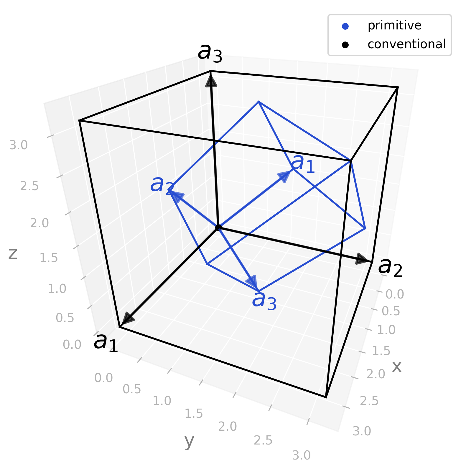
|
import radtools as rad

l = rad.lattice_example(f"FCC")
l.plot(
    "primitive",
    label="primitive",
)
l.legend()
l.plot(
    "conventional",
    label="conventional",
    colour="black"
)
l.legend()
# Save an image:
l.savefig(
    "fcc_real.png",
    elev=28,
    azim=23,
    dpi=300,
   bbox_inches="tight",
)
# Interactive plot:
l.show(elev=28, azim=23)
|
Picture |
Code |
|---|---|
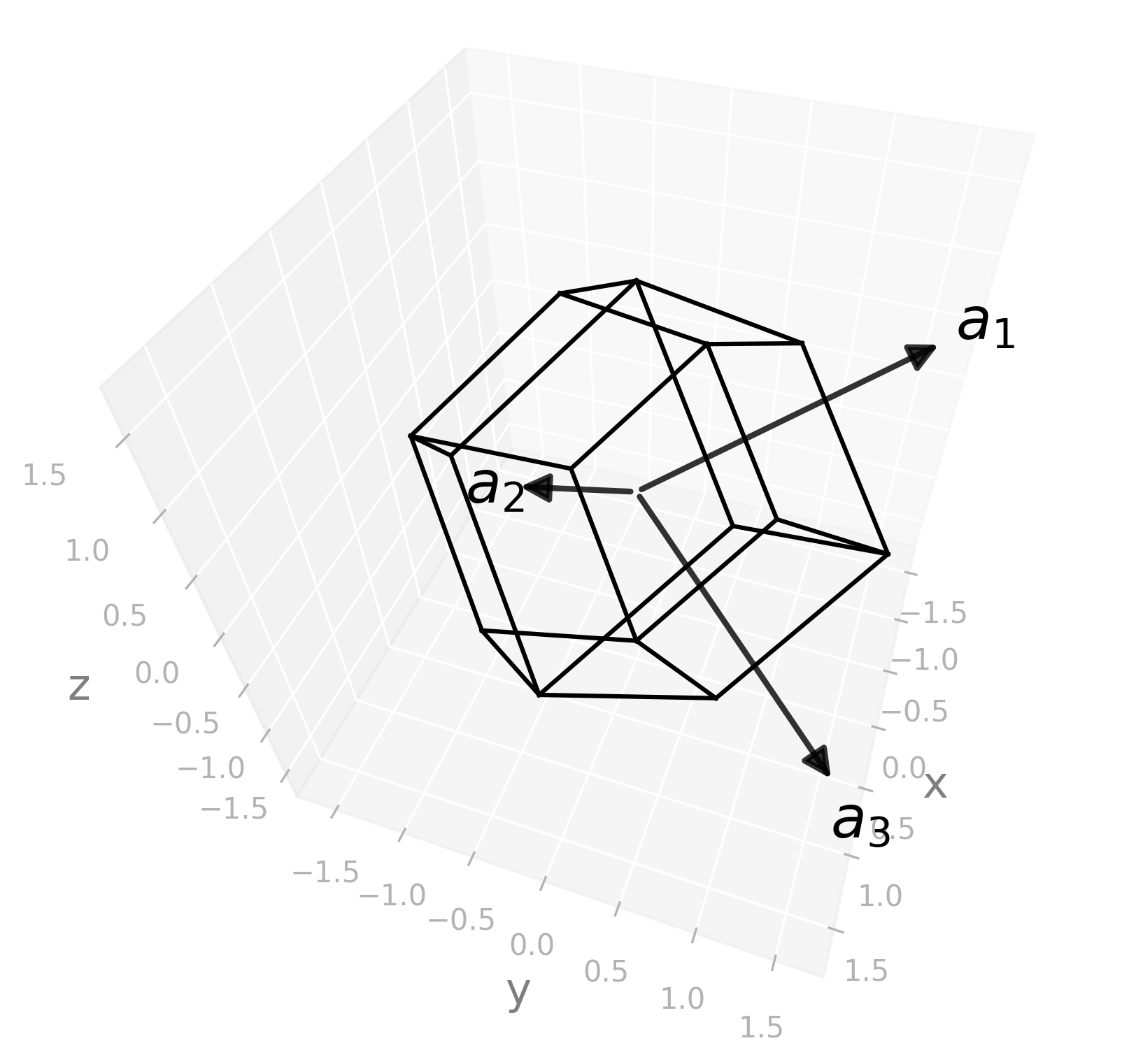
|
import radtools as rad

l = rad.lattice_example(f"FCC")
l.plot("wigner-seitz")
# Save an image:
l.savefig(
    "fcc_wigner-seitz.png",
    elev=46,
    azim=19,
    dpi=300,
   bbox_inches="tight",
)
# Interactive plot:
l.show(elev=46, azim=19)
|