Body-centred orthorhombic (ORCI)#
Pearson symbol: oI
Body-centered orthorombic lattice is described by the class ORCI.
It is defined by three parameter: \(a\), \(b\) and \(c\) with conventional lattice:
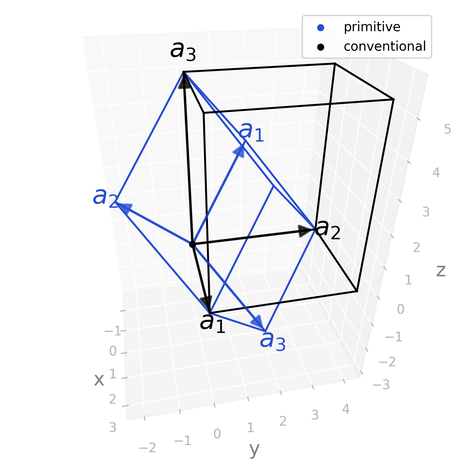
\[ \begin{align}\begin{aligned}\boldsymbol{a}_1 = (a, 0, 0)\\\boldsymbol{a}_2 = (0, b, 0)\\\boldsymbol{a}_3 = (0, 0, c)\end{aligned}\end{align} \]
And primitive lattice:
\[ \begin{align}\begin{aligned}\boldsymbol{a}_1 = (-a/2, b/2, c/2)\\\boldsymbol{a}_2 = (a/2, -b/2, c/2)\\\boldsymbol{a}_3 = (a/2, b/2, -c/2)\end{aligned}\end{align} \]
Order of parameters: \(a < b < c\)
Variations#
There are no variations for body-centered orthorombic.
One example is predefined: orci with
\(a = \pi\), \(b = 1.3\pi\) and \(c = 1.7\pi\).
Example structure#
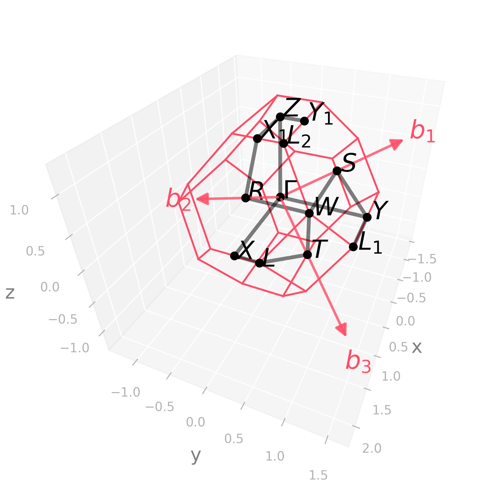
Default kpath: \(\Gamma-X-L-T-W-R-X_1-Z-\Gamma-Y-S-W\vert L_1-Y\vert Y_1-Z\).
Picture |
Code |
|---|---|
|
import radtools as rad

l = rad.lattice_example(f"ORCI")
l.plot("brillouin-kpath")
# Save an image:
l.savefig(
    "orci_brillouin.png",
    elev=35,
    azim=23,
    dpi=300,
   bbox_inches="tight",
)
# Interactive plot:
l.show(elev=35, azim=23)
|
Picture |
Code |
|---|---|
|
import radtools as rad

l = rad.lattice_example(f"ORCI")
l.plot(
    "primitive",
    label="primitive",
)
l.legend()
l.plot(
    "conventional",
    label="conventional",
    colour="black"
)
l.legend()
# Save an image:
l.savefig(
    "orci_real.png",
    elev=32,
    azim=-12,
    dpi=300,
   bbox_inches="tight",
)
# Interactive plot:
l.show(elev=32, azim=-12)
|
Picture |
Code |
|---|---|
|
import radtools as rad

l = rad.lattice_example(f"ORCI")
l.plot("wigner-seitz")
# Save an image:
l.savefig(
    "orci_wigner-seitz.png",
    elev=30,
    azim=12,
    dpi=300,
   bbox_inches="tight",
)
# Interactive plot:
l.show(elev=30, azim=12)
|
Ordering of lattice parameters#
TODO
Edge cases#
If \(a = b \ne c\) or \(a = c \ne b\) or \(b = c \ne a\), then the lattice is Body-centred tetragonal (BCT).
If \(a = b = c\), then the lattice is Body-centered cubic (BCC).