Face-centred orthorhombic (ORCF)#
Pearson symbol: oF
Face-centered orthorombic lattice is described by the class ORCF.
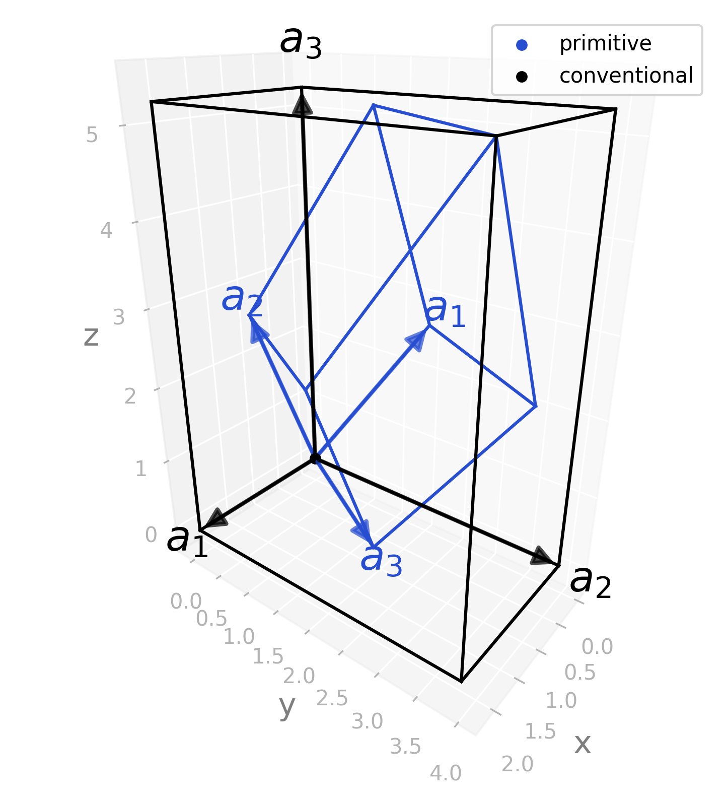
It is defined by three parameters: \(a\), \(b\) and \(c\) with conventional lattice:
And primitive lattice:
Variations#
There are tree variations of face-centered orthorombic lattice.
For the examples of variations \(a\) is set to \(1\); \(b\) and \(c\) fulfil the conditions:
\(b = \dfrac{c}{\sqrt{c^2 - 1}}\)
\(c > \sqrt{2}\)
First condition defines in ORCF3 lattice and ensures ordering of lattice parameters \(b > a\). Ordering \(c > b\) is forced by second condition.
For ORCF1 and ORCF2 lattices \(a < 1\) and \(a > 1\) is chosen. While \(b\) and \(c\) are the same as for ORCF3 lattice.
At the end all three parameters are multiplied by \(\pi\).
ORCF1#
\(\dfrac{1}{a^2} > \dfrac{1}{b^2} + \dfrac{1}{c^2}\).
Predefined example: orcf1 with
\(a = 0.7\pi\), \(b = 5\pi/4\) and \(c = 5\pi/3\).
ORCF2#
\(\dfrac{1}{a^2} < \dfrac{1}{b^2} + \dfrac{1}{c^2}\).
Predefined example: orcf2 with
\(a = 1.2\pi\), \(b = 5\pi/4\) and \(c = 5\pi/3\).
ORCF3#
\(\dfrac{1}{a^2} = \dfrac{1}{b^2} + \dfrac{1}{c^2}\).
Predefined example: orcf3 with
\(a = \pi\), \(b = 5\pi/4\) and \(c = 5\pi/3\).
Example structures#
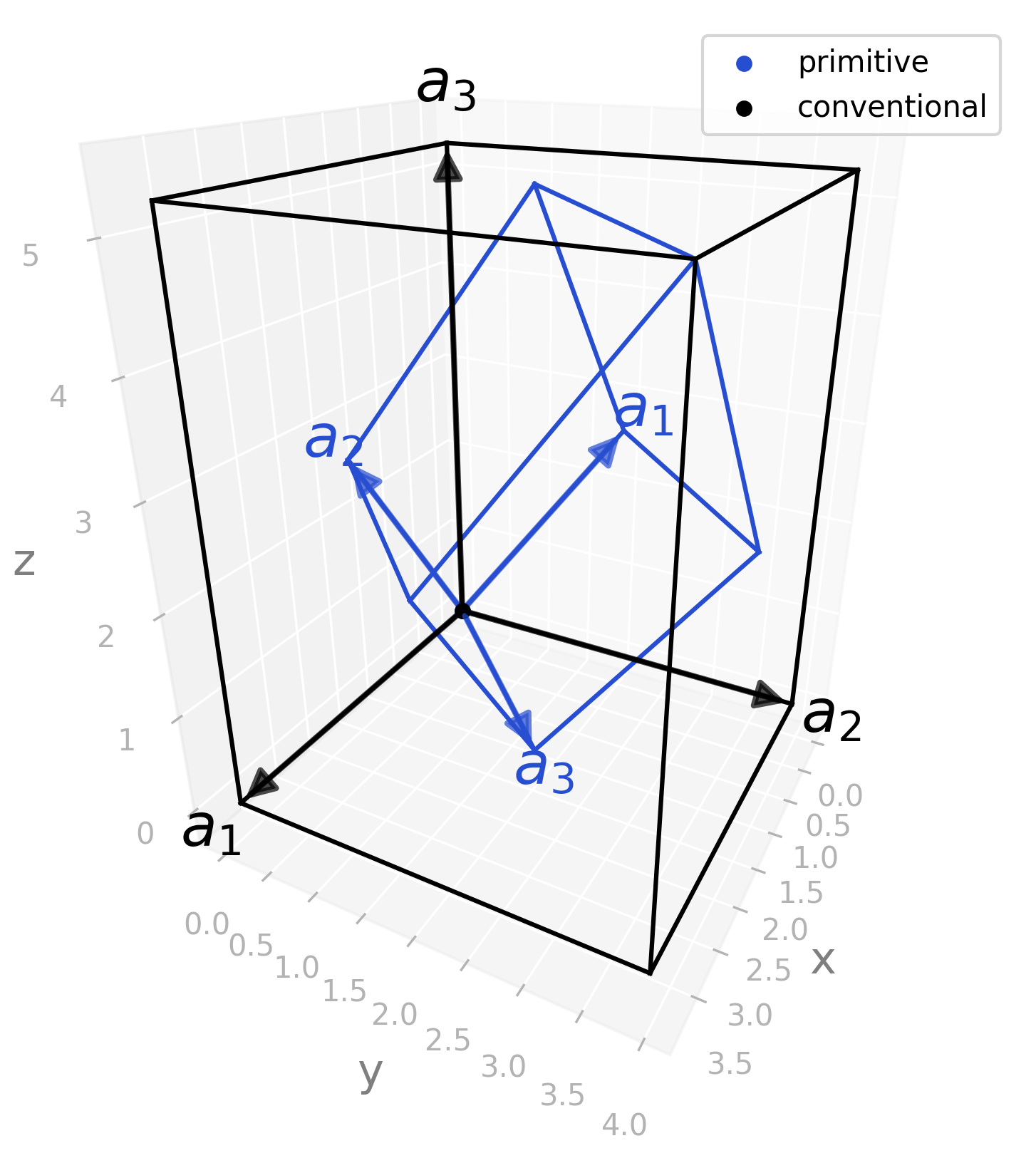
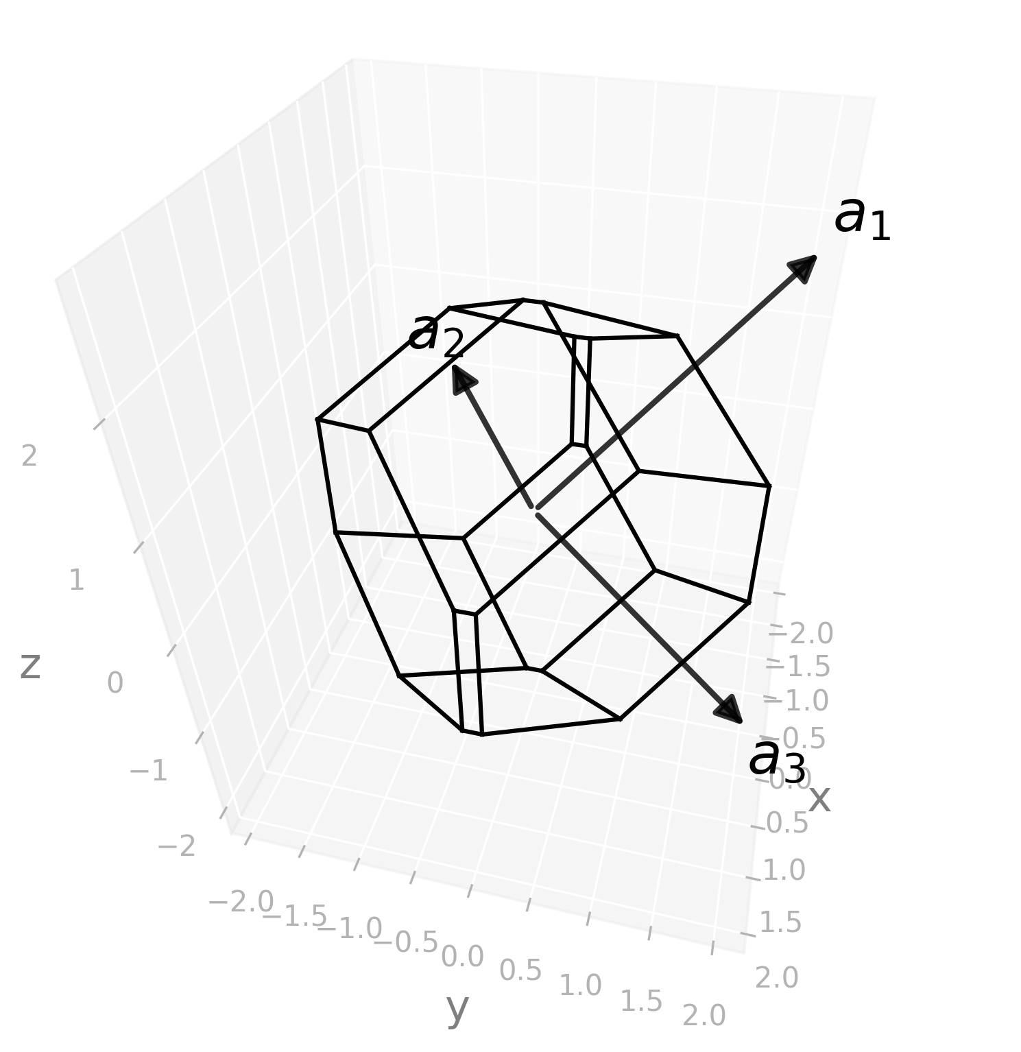
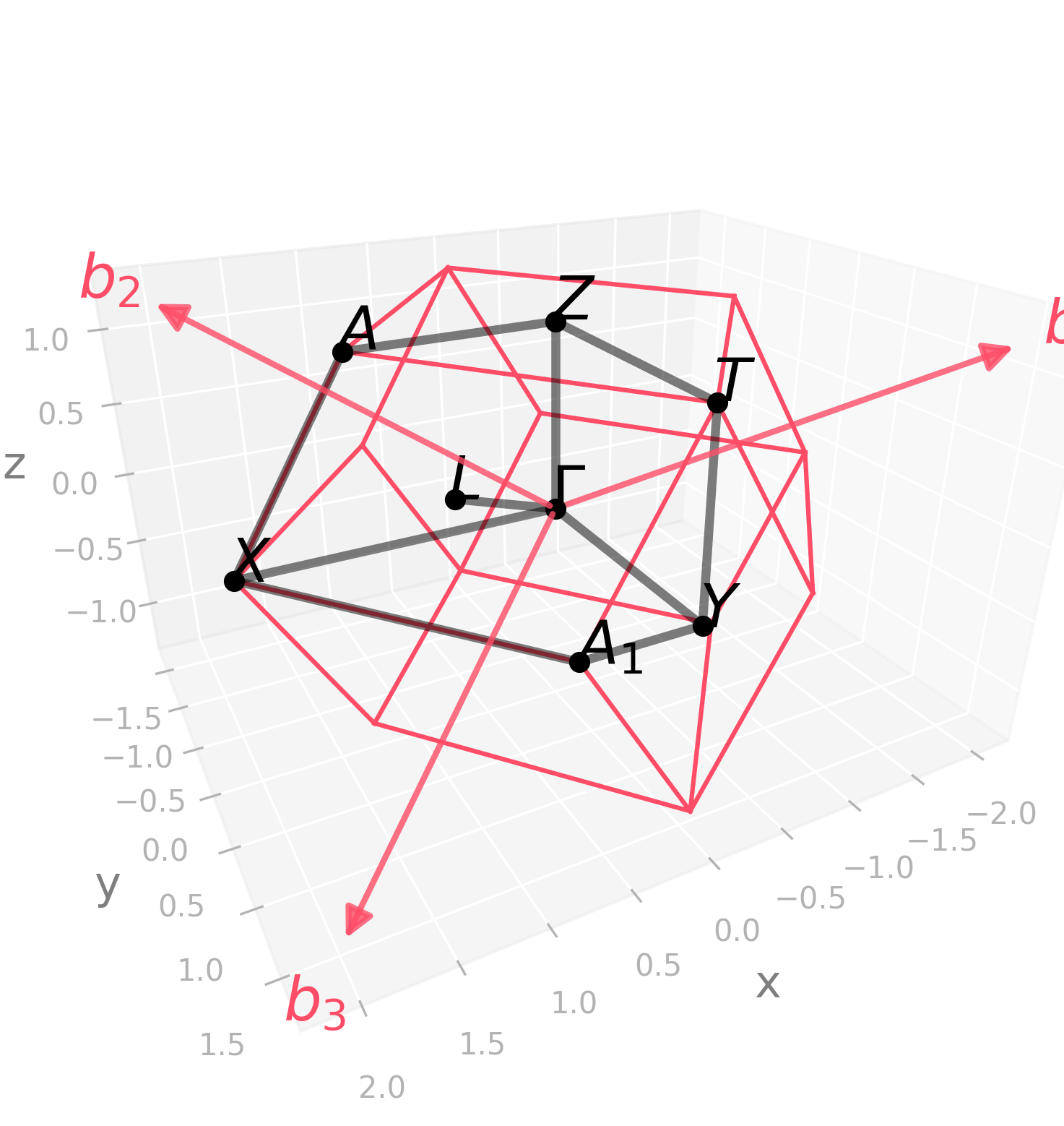
ORCF1#
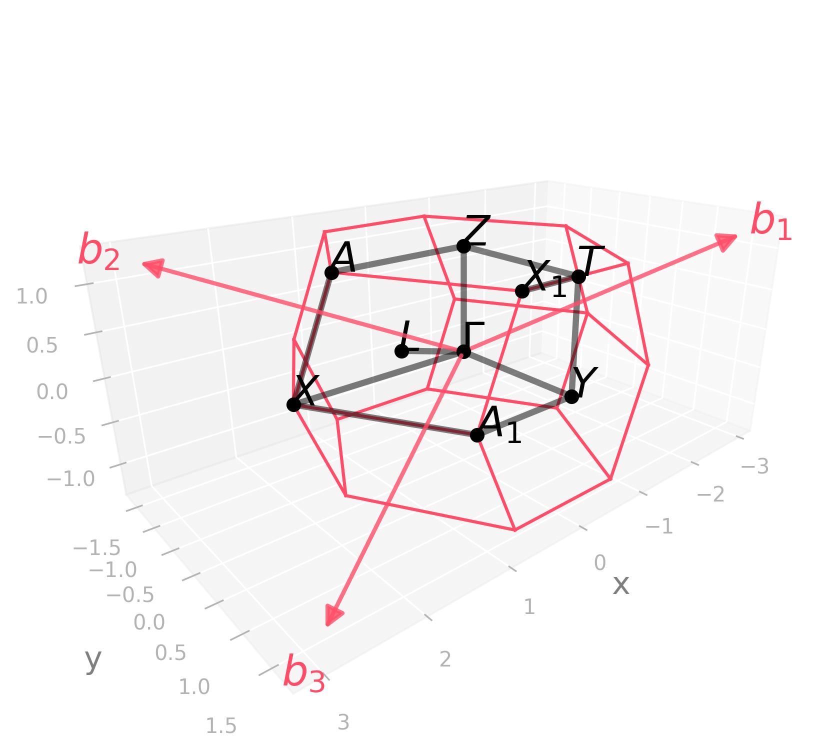
Default kpath: \(\Gamma-Y-T-Z-\Gamma-X-A_1-Y\vert T-X_1\vert X-A-Z\vert L-\Gamma\).
Picture |
Code |
|---|---|
|
import radtools as rad

l = rad.lattice_example(f"ORCF1")
l.plot("brillouin-kpath")
# Save an image:
l.savefig(
    "orcf1_brillouin.png",
    elev=21,
    azim=49,
    dpi=300,
   bbox_inches="tight",
)
# Interactive plot:
l.show(elev=21, azim=49)
|
Picture |
Code |
|---|---|
|
import radtools as rad

l = rad.lattice_example(f"ORCF1")
l.plot(
    "primitive",
    label="primitive",
)
l.legend()
l.plot(
    "conventional",
    label="conventional",
    colour="black"
)
l.legend()
# Save an image:
l.savefig(
    "orcf1_real.png",
    elev=24,
    azim=38,
    dpi=300,
   bbox_inches="tight",
)
# Interactive plot:
l.show(elev=24, azim=38)
|
Picture |
Code |
|---|---|
|
import radtools as rad
l = rad.lattice_example(f"ORCF1")
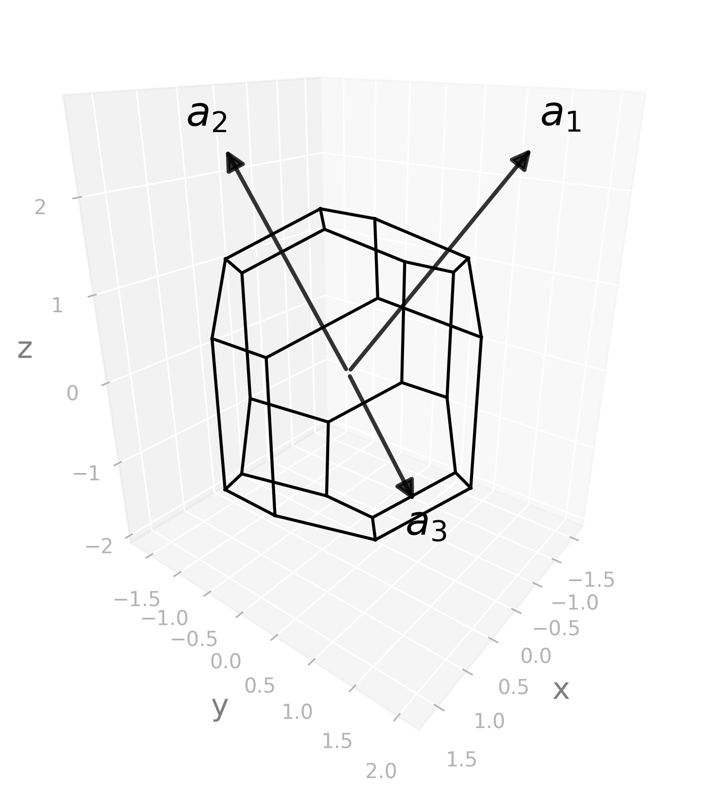
l.plot("wigner-seitz")
# Save an image:
l.savefig(
"orcf1_wigner-seitz.png",
elev=44,
azim=28,
dpi=300,
bbox_inches="tight",
)
# Interactive plot:
l.show(elev=44, azim=28)
|
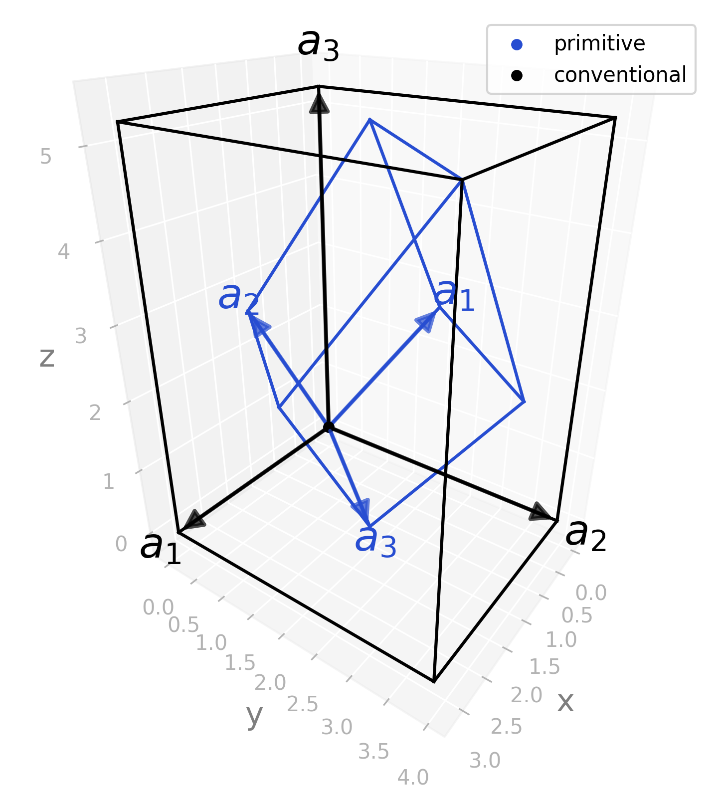
ORCF2#
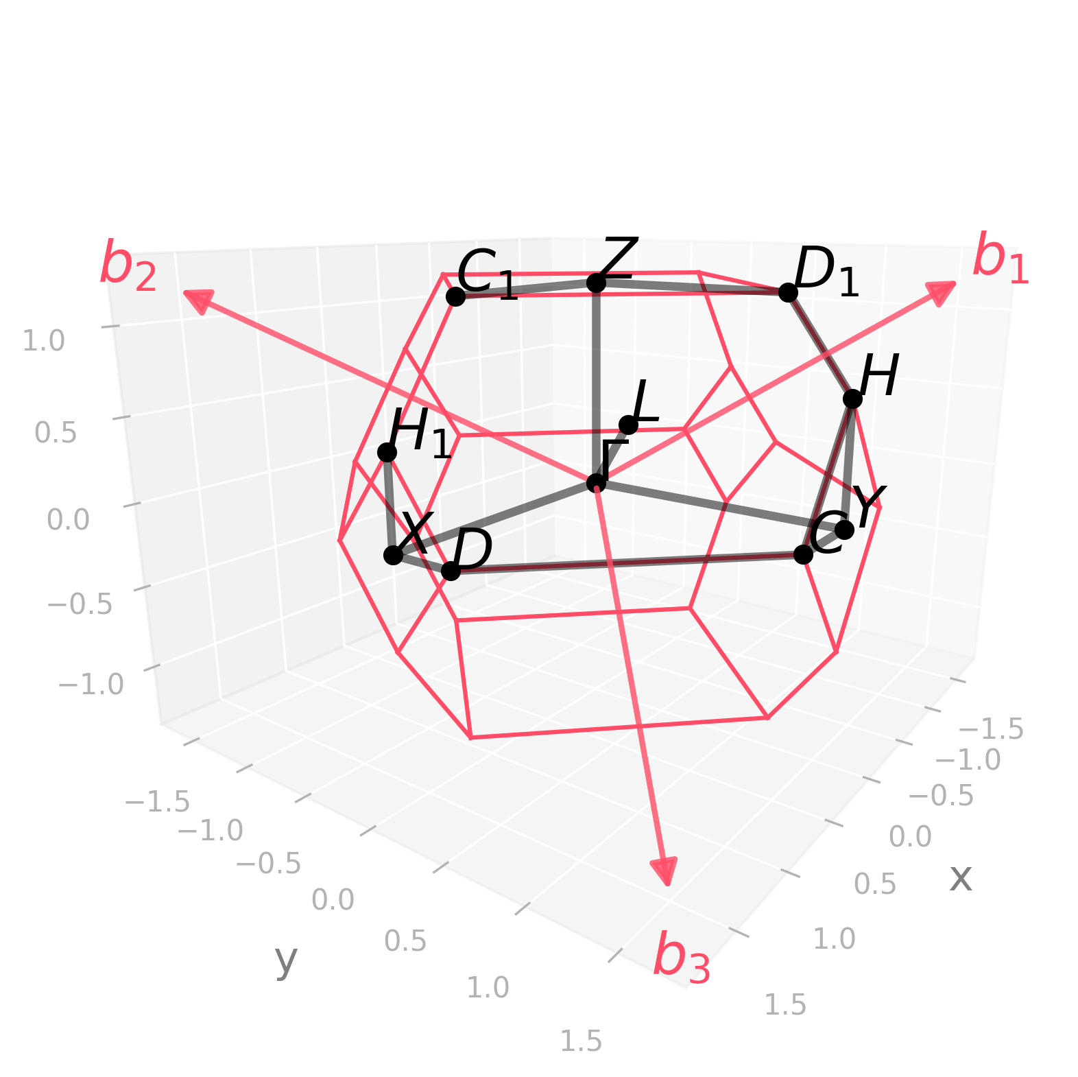
Default kpath: \(\Gamma-Y-C-D-X-\Gamma-Z-D_1-H-C\vert C_1-Z\vert X-H_1\vert H-Y\vert L-\Gamma\).
Picture |
Code |
|---|---|
|
import radtools as rad

l = rad.lattice_example(f"ORCF2")
l.plot("brillouin-kpath")
# Save an image:
l.savefig(
    "orcf2_brillouin.png",
    elev=15,
    azim=36,
    dpi=300,
   bbox_inches="tight",
)
# Interactive plot:
l.show(elev=15, azim=36)
|
Picture |
Code |
|---|---|
|
import radtools as rad

l = rad.lattice_example(f"ORCF2")
l.plot(
    "primitive",
    label="primitive",
)
l.legend()
l.plot(
    "conventional",
    label="conventional",
    colour="black"
)
l.legend()
# Save an image:
l.savefig(
    "orcf2_real.png",
    elev=25,
    azim=28,
    dpi=300,
   bbox_inches="tight",
)
# Interactive plot:
l.show(elev=25, azim=28)
|
Picture |
Code |
|---|---|
|
import radtools as rad

l = rad.lattice_example(f"ORCF2")
l.plot("wigner-seitz")
# Save an image:
l.savefig(
    "orcf2_wigner-seitz.png",
    elev=38,
    azim=14,
    dpi=300,
   bbox_inches="tight",
)
# Interactive plot:
l.show(elev=38, azim=14)
|
ORCF3#
Default kpath: \(\Gamma-Y-T-Z-\Gamma-X-A_1-Y\vert X-A-Z\vert L-\Gamma\).
Picture |
Code |
|---|---|
|
import radtools as rad

l = rad.lattice_example(f"ORCF3")
l.plot("brillouin-kpath")
# Save an image:
l.savefig(
    "orcf3_brillouin.png",
    elev=25,
    azim=62,
    dpi=300,
   bbox_inches="tight",
)
# Interactive plot:
l.show(elev=25, azim=62)
|
Picture |
Code |
|---|---|
|
import radtools as rad

l = rad.lattice_example(f"ORCF3")
l.plot(
    "primitive",
    label="primitive",
)
l.legend()
l.plot(
    "conventional",
    label="conventional",
    colour="black"
)
l.legend()
# Save an image:
l.savefig(
    "orcf3_real.png",
    elev=27,
    azim=36,
    dpi=300,
   bbox_inches="tight",
)
# Interactive plot:
l.show(elev=27, azim=36)
|
Picture |
Code |
|---|---|
|
import radtools as rad

l = rad.lattice_example(f"ORCF3")
l.plot("wigner-seitz")
# Save an image:
l.savefig(
    "orcf3_wigner-seitz.png",
    elev=23,
    azim=38,
    dpi=300,
   bbox_inches="tight",
)
# Interactive plot:
l.show(elev=23, azim=38)
|
Ordering of lattice parameters#
TODO
Edge cases#
If \(a = b \ne c\) or \(a = c \ne b\) or \(b = c \ne a\), then the lattice is Body-centred tetragonal (BCT).
If \(a = b = c\), then the lattice is Face-centred cubic (FCC).