Orthorhombic (ORC)#
Pearson symbol: oP
Orthorombic lattice is described by the class ORC.
It is defined by three parameter: \(a\), \(b\) and \(c\) with primitive and conventional lattice:
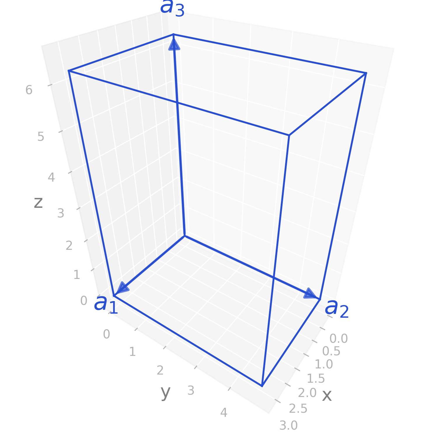
\[ \begin{align}\begin{aligned}\boldsymbol{a}_1 = (a, 0, 0)\\\boldsymbol{a}_2 = (0, b, 0)\\\boldsymbol{a}_3 = (0, 0, c)\end{aligned}\end{align} \]
Order of parameters: \(a < b < c\)
Variations#
There are no variations for orthorhombic lattice.
One example is predefined: orc with
\(a = \pi\), \(b = 1.5\pi\) and \(c = 2\pi\).
Example structure#
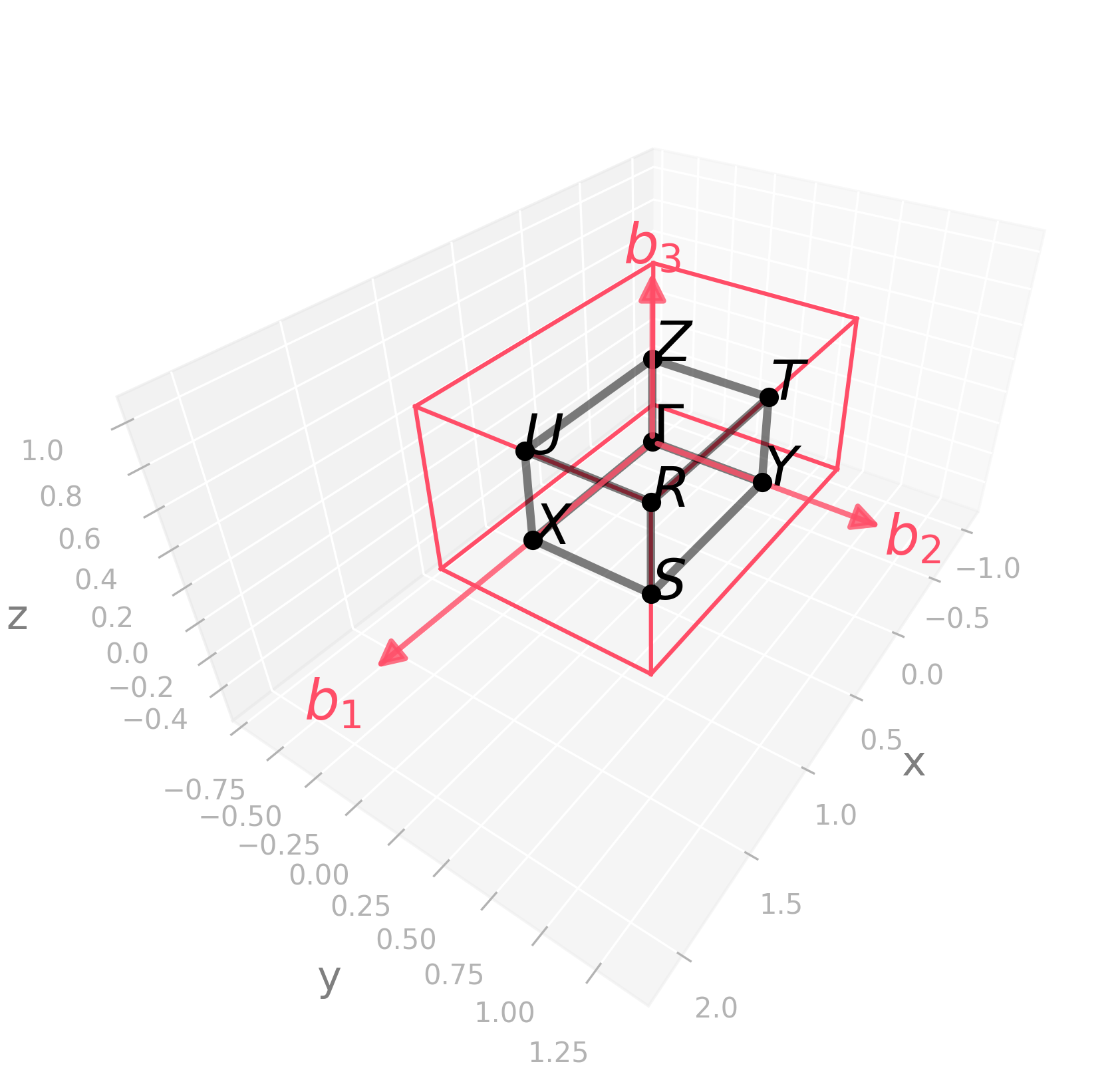
Default kpath: \(\Gamma-X-S-Y-\Gamma-Z-U-R-T-Z\vert Y-T\vert U-X\vert S-R\).
Picture |
Code |
|---|---|
|
import radtools as rad

l = rad.lattice_example(f"ORC")
l.plot("brillouin-kpath")
# Save an image:
l.savefig(
    "orc_brillouin.png",
    elev=35,
    azim=34,
    dpi=300,
   bbox_inches="tight",
)
# Interactive plot:
l.show(elev=35, azim=34)
|
Picture |
Code |
|---|---|
|
import radtools as rad

l = rad.lattice_example(f"ORC")
l.plot("primitive")
# Save an image:
l.savefig(
    "orc_real.png",
    elev=36,
    azim=35,
    dpi=300,
   bbox_inches="tight",
)
# Interactive plot:
l.show(elev=36, azim=35)
|
Picture |
Code |
|---|---|
|
import radtools as rad

l = rad.lattice_example(f"ORC")
l.plot("wigner-seitz")
# Save an image:
l.savefig(
    "orc_wigner-seitz.png",
    elev=20,
    azim=30,
    dpi=300,
   bbox_inches="tight",
)
# Interactive plot:
l.show(elev=20, azim=30)
|
Ordering of lattice parameters#
TODO
Edge cases#
If \(a = b \ne c\) or \(a = c \ne b\) or \(b = c \ne a\), then the lattice is Tetragonal (TET).
If \(a = b = c\), then the lattice is Cubic (CUB).