Rhombohedral (RHL)

Pearson symbol: hR

Rhombohedral lattice is described by the class RHL.

It is defined by two parameter: \(a\) and \(\alpha\) with primitive and conventional lattice:

\[ \begin{align}\begin{aligned}\boldsymbol{a}_1 = (a\cos(\alpha / 2), -a\sin(\alpha/2), 0)\\\boldsymbol{a}_2 = (a\cos(\alpha / 2), a\sin(\alpha/2), 0)\\\boldsymbol{a}_3 = \left(\frac{\cos(\alpha)}{\cos(\alpha/2)}, 0, a\sqrt{1 - \frac{\cos^2(\alpha)}{\cos^2(\alpha/2)}}\right)\end{aligned}\end{align} \]

Variations

There are two variations for rhombohedral lattice.

RHL₁

\(\alpha < 90^{\circ}\).

Predefined example: rhl1 with \(a = \pi\) and \(\alpha = 70\)

RHL₂

\(\alpha > 90^{\circ}\).

Predefined example: rhl2 with \(a = \pi\) and \(\alpha = 110\)

Example structure

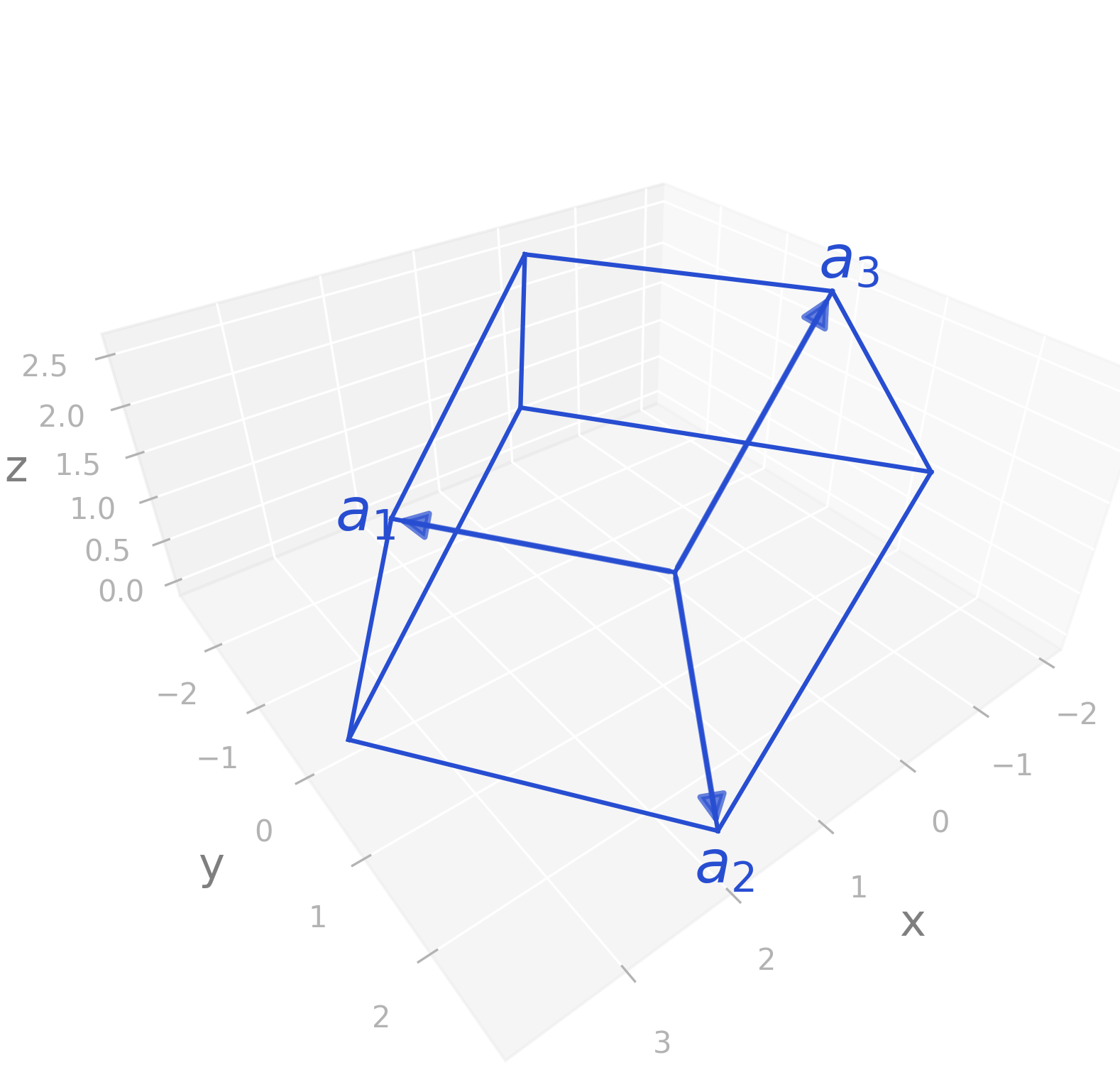
RHL₁

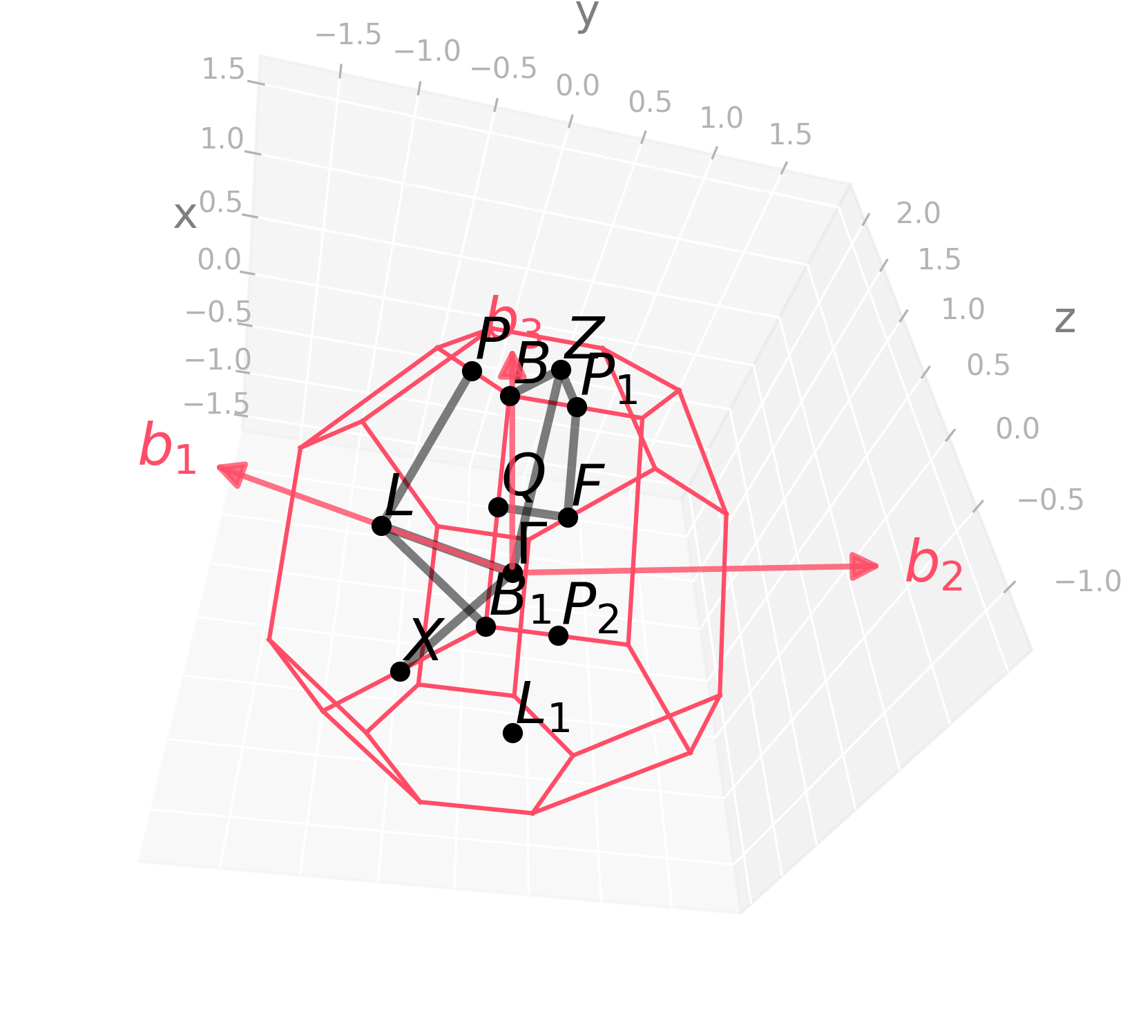
Default kpath: \(\Gamma-L-B_1\vert B-Z-\Gamma-X\vert Q-F-P_1-Z\vert L-P\).

Brillouin zone and default kpath

Picture	Code
	import radtools as rad l = rad.lattice_example(f"RHL1") l.plot("brillouin-kpath") # Save an image: l.savefig( "rhl1_brillouin.png", elev=-41, azim=-13, dpi=300, bbox_inches="tight", ) # Interactive plot: l.show(elev=-41, azim=-13)

Primitive and conventional cell

Picture	Code
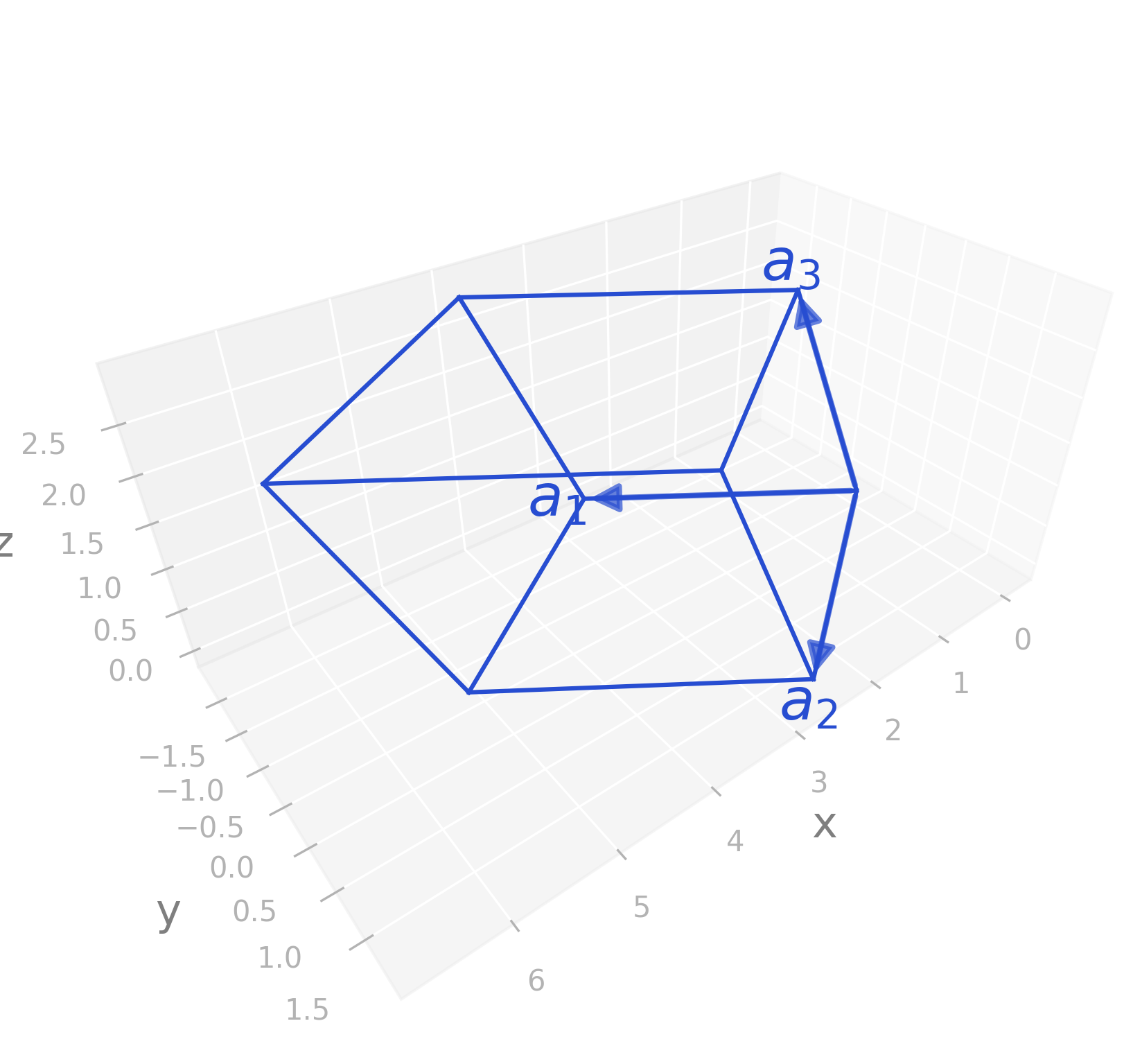
	import radtools as rad l = rad.lattice_example(f"RHL1") l.plot("primitive") # Save an image: l.savefig( "rhl1_real.png", elev=35, azim=52, dpi=300, bbox_inches="tight", ) # Interactive plot: l.show(elev=35, azim=52)

Wigner-Seitz cell

Picture	Code
	import radtools as rad l = rad.lattice_example(f"RHL1") l.plot("wigner-seitz") # Save an image: l.savefig( "rhl1_wigner-seitz.png", elev=19, azim=-19, dpi=300, bbox_inches="tight", ) # Interactive plot: l.show(elev=19, azim=-19)

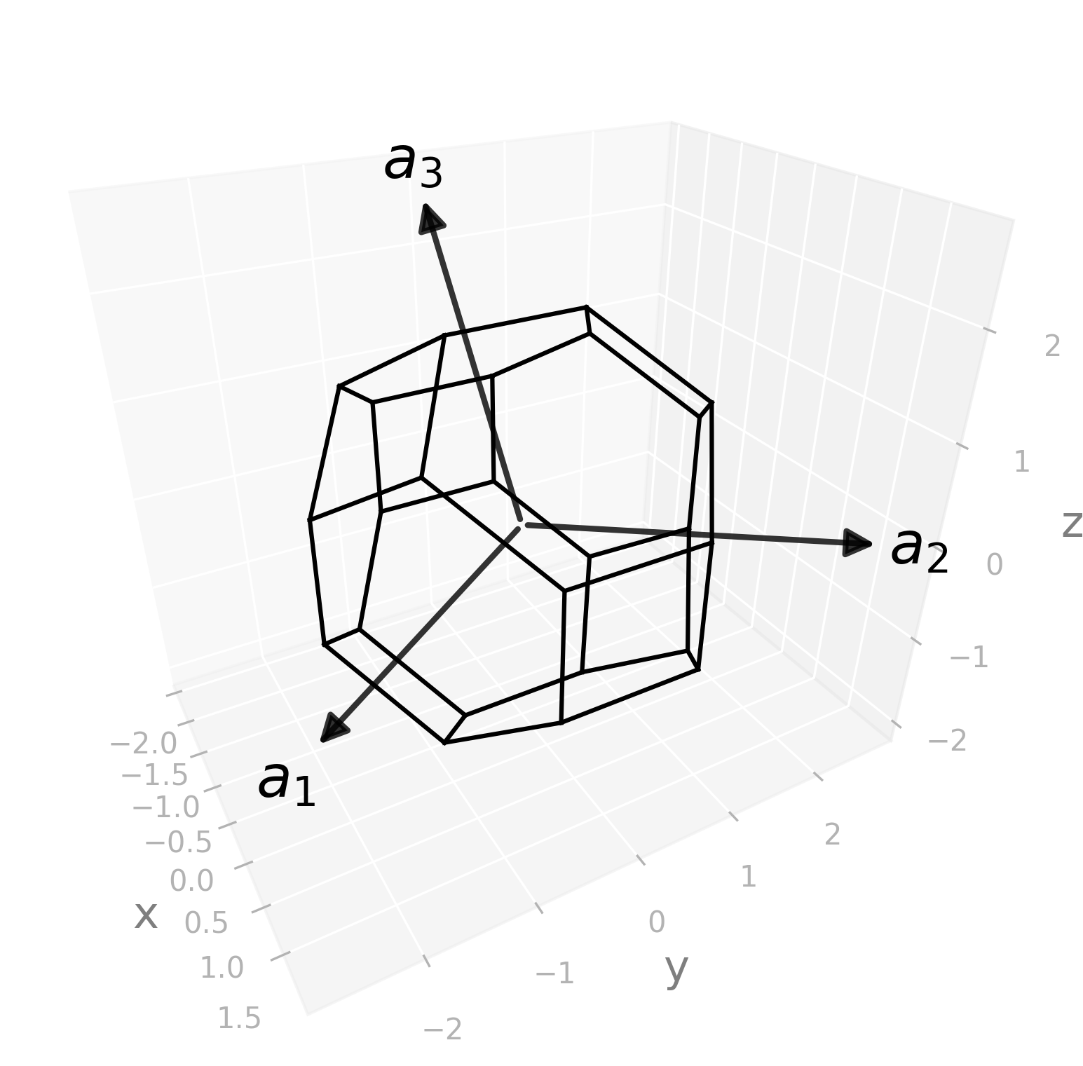
RHL₂

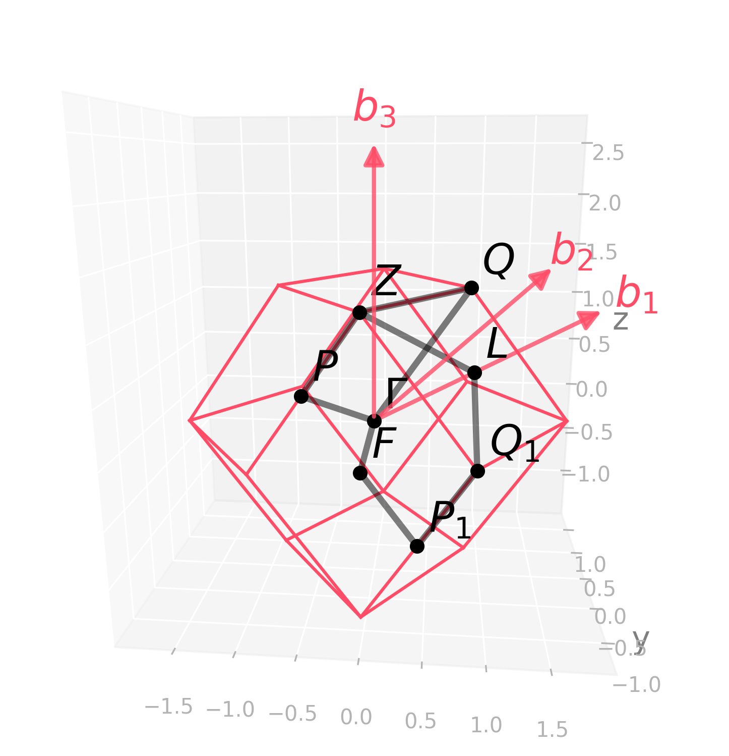
Default kpath: \(\Gamma-P-Z-Q-\Gamma-F-P_1-Q_1-L-Z\).

Brillouin zone and default kpath

Picture	Code
	import radtools as rad l = rad.lattice_example(f"RHL2") l.plot("brillouin-kpath") # Save an image: l.savefig( "rhl2_brillouin.png", elev=14, azim=-85, dpi=300, bbox_inches="tight", ) # Interactive plot: l.show(elev=14, azim=-85)

Primitive and conventional cell

Picture	Code
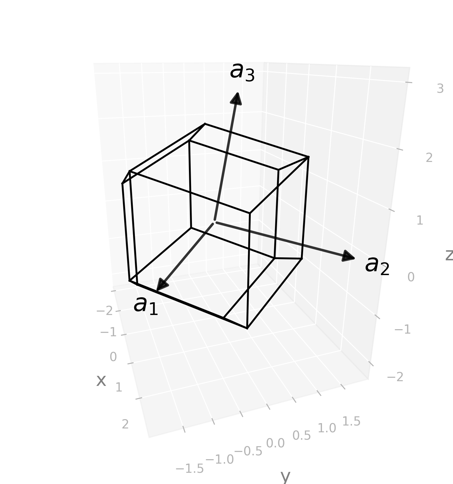
	import radtools as rad l = rad.lattice_example(f"RHL2") l.plot("primitive") # Save an image: l.savefig( "rhl2_real.png", elev=35, azim=52, dpi=300, bbox_inches="tight", ) # Interactive plot: l.show(elev=35, azim=52)

Wigner-Seitz cell

Picture	Code
	import radtools as rad l = rad.lattice_example(f"RHL2") l.plot("wigner-seitz") # Save an image: l.savefig( "rhl2_wigner-seitz.png", elev=30, azim=-29, dpi=300, bbox_inches="tight", ) # Interactive plot: l.show(elev=30, azim=-29)

Edge cases

In rhombohedral lattice \(a = b = c\) and \(\alpha = \beta = \gamma\), thus three edge cases exist:

If \(\alpha = 60^{\circ}\), then the lattice is Face-centred cubic (FCC)

If \(\alpha \approx 109.47122063^{\circ}\) (\(\cos(\alpha) = -1/3\)), then the lattice is Body-centered cubic (BCC).

If \(\alpha = 90^{\circ}\), then the lattice is Cubic (CUB).